Before it gets messy

Discovering the Solver node: creating a Pseudo-Voronoï fracture and some cool waves

These past days, when playing with Houdini, I was somehow really frustrated because I could not use the previous frames as input to create some faked dynamics inside my geometry block. Of course, since it’s basically for creating dynamics, I could take a look at DOPs but I don’t feel quite ready for that yet (too complicated, I’m such a slow learner).

So, I looked a little bit in the doc, the internet and tested some nodes and I found out the Node ‘Solver’ which basically does exactly what I wanted!

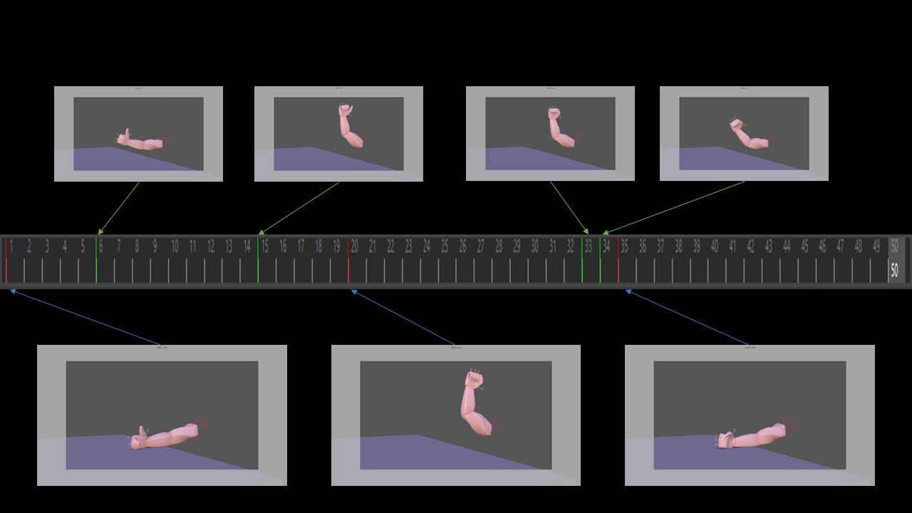
Let’s start with showing the result of today’s practice

Let me just explain quickly what it’s all about. I’m starting with a point cloud where all the clouds are neutral except a few (the colored ones). At each frame, the colorful points try to contaminate their neighbours according to a procedure that I describe below. Then, I use the time of contamination to drive a cosine displacement along the normals which creates a wavy effect.

In the upcoming paragraph I will give a breakdown of the process; in the last paragraph, I will speak a little bit about mathematics and geometry (basically, my results can somehow look like Voronoï fracture and I’m trying to give an intuition of ‘why’). I might be getting things wrong, so, as always, do not hesitate to contact me for improvement or questions!

Step 0: preparing the data

Just saying, I will apply everything to a point cloud that I will create by scattering points along a surface. Indeed, the displacement along the normals make sense only if I have normals to start with so scattering along a surface and not a density makes more sense:

Put it that way, that’s probably more clear ^^

Step 1: Contamination

Basically, I’m creating clusters via a contamination process. The idea is as followed: I have some points that are contaminated. They will ocntaminate their neighbours at each frame so the contaminated part will eventually grow and all the points will be contaminated in the end. The results can change a lot depending on what the contamination procedure consists of so I’m going to explain it right now!

Of course, there are plenty of ways to define this step (and I will discuss it a little bit later) but this one is interesting because it can create some artifacts and is really easy to code -that was just a test after all 😀

The network for Step 1!
Notice the green clocks: it means that, at those nodes, the geometry is animated!

Step 1.1 Initializing

Sorry, but you have to read like a manga, first wrangle is the right one -_-

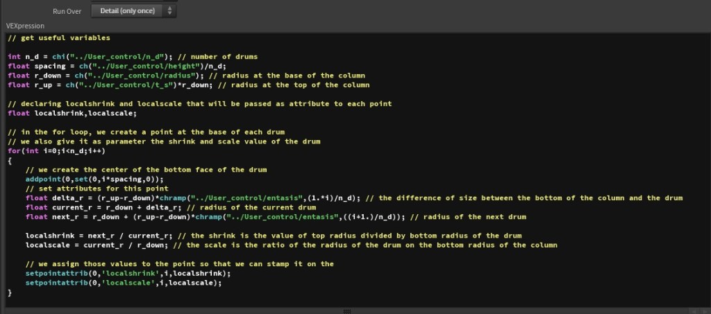
The create_attrib wrangle creates where we will store the ID of the cluster each point belongs in and a birthdate value which corresponds to the distance (in term of contamination) from the point to the origin of the contamination. The ID of a neutral point is -1. The initialize wrangle will pick a random starting point for each cluster.

Step 1.2 Solver!!!!!

Now, let’s talk about our main interest: the Solver node. To use this guy properly, you first need to double click to enter into it and discovers its secret:

Initially there was only the purple node, I added 2 wrangles after

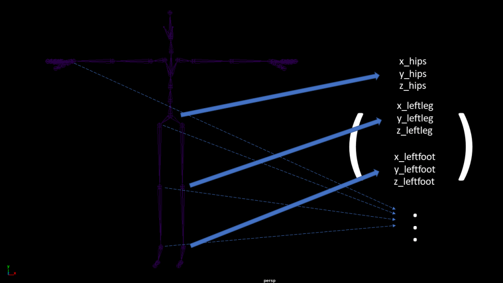
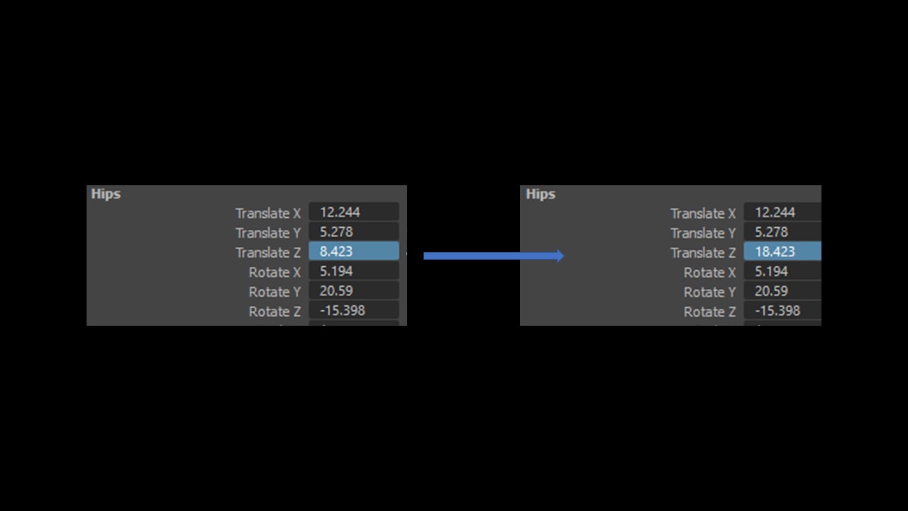
Basically, it’s the purple node that does the magic: using it, you can access your geometry parameters in the state they were one frame before. So for example if I write this:

@P.y += 1;

In a wrangle outside of the solver, it will just move my geometry of 1 unit along the y-axis and nothing more. But if I put this wrangle inside the Solver, the geometry will move of 1 more unit incrementaly at each frame!

Here’s what inside our ‘expansion’ wrangle

It is a simple implementation of the rules I stated before. If you pay a close attention, I am not setting directly the attribute ‘cluster’ but an auxiliary attribute called ‘next_cluster’. I don’t really know how Houdini operates the parallel operations so I want first to get how I will change my points then change them ONLY when I figured out ALL the values I need to change (If by any chance you have infos on how Houdini parallelize the computations I would be really delighted to hear from you!). And that’s why I have a wrangle ‘update’ that will do exactly this:

And that’s all

Step 1.3 Setting colors

That’s just straightforward: set a color for each cluster and assign the right color to the right points:

I assign color c[i] to points of cluster i

Step 2. Making waves

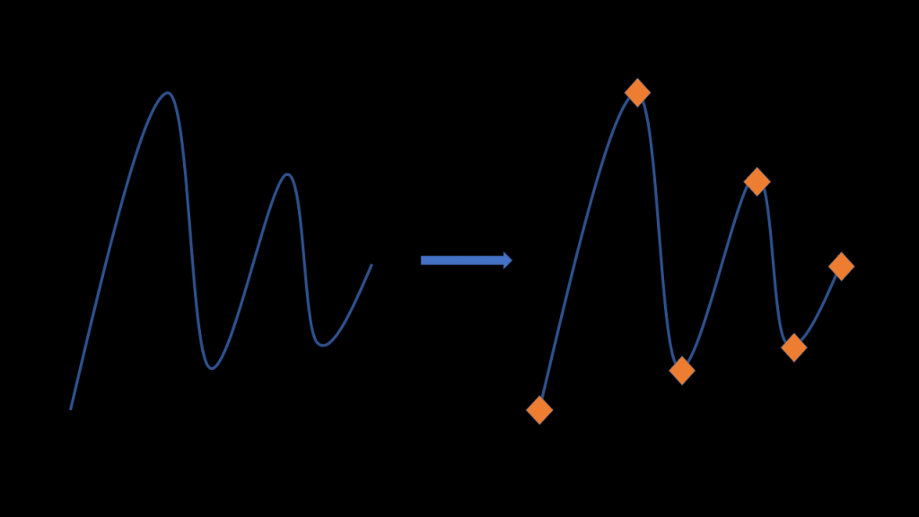
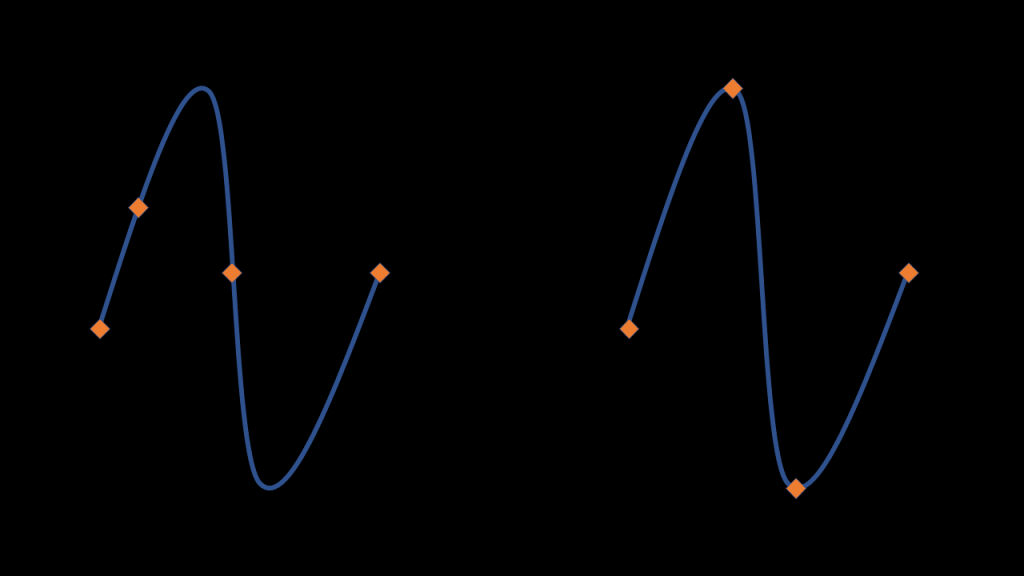
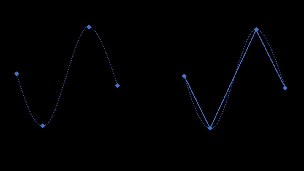
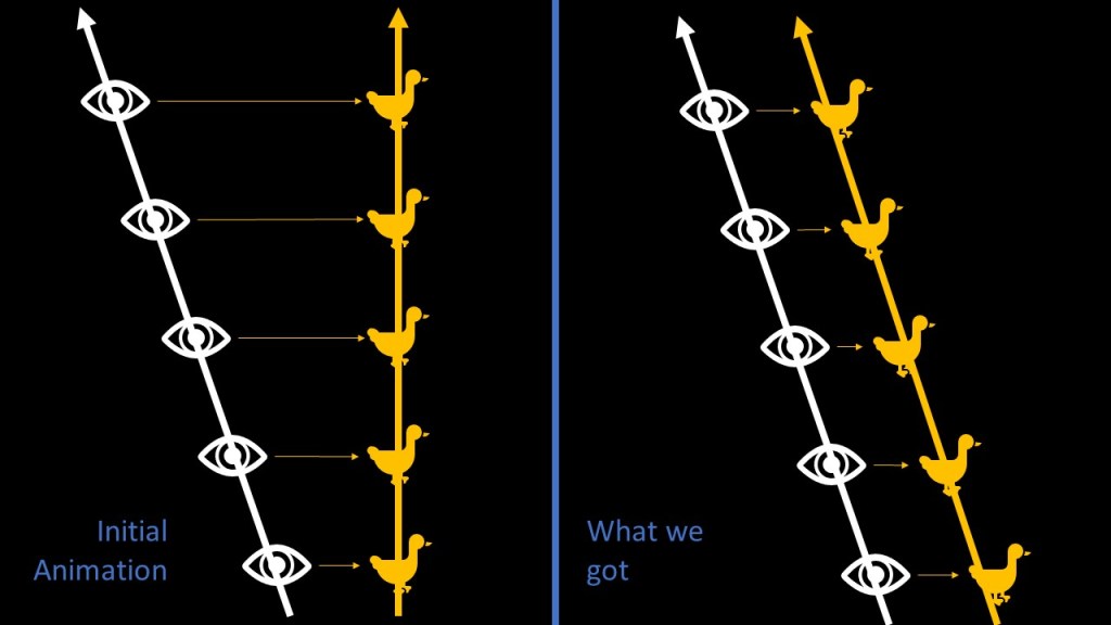
This step was totally unnecessary but I find it pretty cool so I did it. Creating a wavy effect is pretty easy, most of the time you can achieve it by displacing along the normals with a cosine signal. But if you do not take anything else into account, everything will bounce at the same rythm and it will not create any waves.

To solve this problem, a standard way to do would be to choose a point as an origin for the waves and then multiply the displacement by the cosine of the distance between the current point and the origin. So, to make it short, having 2 sinusoidal signals, one in terms of time, the other in terms of position.

Here, rather than using directly the Euclidean distance (i.e the usual distance), I prefer using the birthdate (i.e the date of contamination) of our point. Actually, there’s a mathematical meaning to do that (I am not doing nonsense) that I explain in the next paragraph if you are interested.

‘internal_frequency’ must be understood as ‘spatial frequency’ while ‘frequency’ is ‘temporal frequency’

Let’s talk math shall we?

What is interesting about this short example is that it lets me introduce some maths. Actually, there are 2 things I want to talk about: metrics and Voronoi diagrams.

Why does it make sense to use the birthdate in place of the distance for the temporal sinusoidal signal?

Short answer is: because we can define a pseudometric from it (basically, it means that it implements a notion of distance)

The way I am creating the contamination can be represented as a tree:

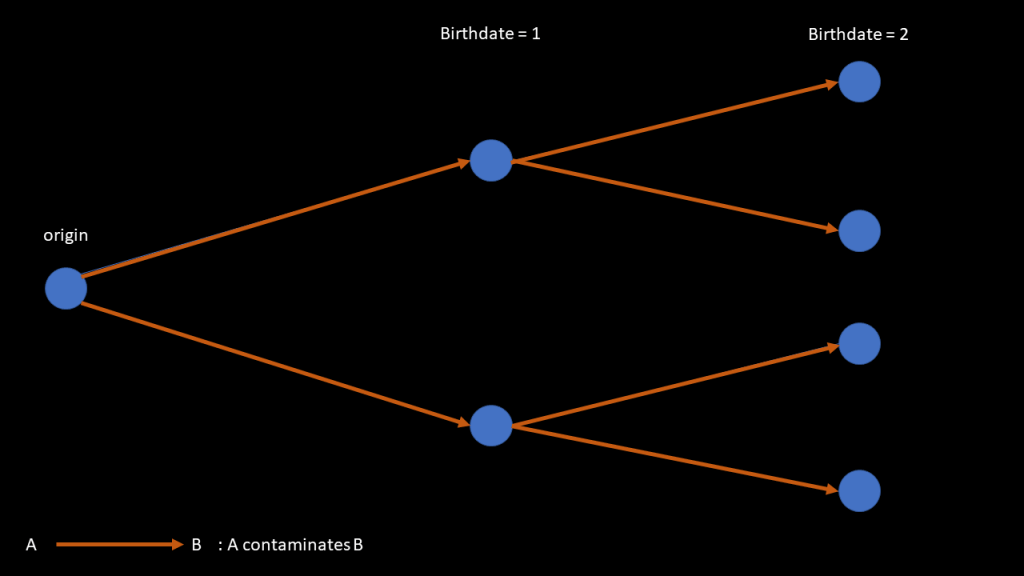
And I can define a pseudodistance for the elements of that tree by taking the difference of their birthdate: $d(x,y)=abs(birthdate_x-birthdate_y)$ . What is a pseudodistance though?

So, a distance is used to evaluate how 2 points are far one from each other. A pseudodistance is merely the same, except that it fails at distinguishing 2 points: for a distance $d(x,y)=0$ means that $x=y$ while it is not the case for a pseudodistance. (check here for the mathematical properties. Proof that the difference in birthdate is a pseudo-distance is left to the reader lol)

So, even though my choice of using the birthdate was mainly driven by my laziness, it still made sense mathematically and was in some way even a better choice than using the Euclidean distance. Indeed, the Euclidean distance does not take into account at all the shape of my surface, while it is the case for my pseudo-distance (best case scenario would be to use a geodesic distance along the surface, but that’s hard to implement and to keep good performance using that).

About Voronoï fracture/diagrams

If you are used to play with Voronoï fractures in Houdini or with Voronoï diagrams in computational geometry, you probably have noticed that the clusters created by my thingy somehow look like Voronoï cells. And, guess what, it is not a coincidence.

Let me first recall you what a Voronoï diagram is (I’ll try to make a whole note about it later on because a short explanation might be confusing).

A 2D Voronoi diagram (credits: Wikipédia)

Notice that all cells only contain one black point that we call a seed. Basically, to obtain this diagram, first, I give you the seeds. Then, given a seed, its cell is the set of points that are closer to this seed than to any other seeds.

With our method, the closer a point is from the center of a cluster, the more likely it will belong to this cluster. So, a cluster will be approximately the set of points that are closer to the origin of this cluster than any other origins. And Iif you followed what I said earlier, it really looks like the definition of the Voronoi diagram. Which explains why it is so similar with the regular Voronoi diagram.

Our method is kinda doing this, but with a more chaotic approach, so it’s normal we ‘somehow’ get a similar result! (credits: Wikipédia)

A more ‘advanced’ point of view regarding the Voronoi similarity

Thing is, the clustering we obtain is also a Voronoi diagram but with another distance. When I said ‘closer’ earlier, I immediately implied that there is an underlying notion of distance. In most cases, we stick to the Euclidean distance but we do not necessarily have to.

Indeed, I can define an asymmetric distance on my set of points by defining $d(x,y)$ as the time it will take to contaminate x, starting from y, with the given procedure. We can prove it is defined, and verifies all the distance properties except the symmetry (ask me if you want the proof).

With this distance as the underlying metric, our algorithm exactly boils down to draw the Voronoi diagram! To be perfectly honest, I’m not sure how it is a relevant information though, as it sounds more like a tautology than anything but that’s cool anyway XD

Quick Columns with Revolve

I presented in my Houdini series a whole paragraph about building columns. Fact is, it was somehow complicated and performances are pretty bad as we accumulate for-loops in VEX wrangles.

If you just want the shape of a column and do not care at all about all the flutes and stuff, here is a super simple set-up to create your column (but can be used to design bowls or such) that just uses 2 (or 3) nodes.

First we create a curve thanks to an Attribute Wrangle (can also use Houdini’s curve but you need to draw it in the viewport. I personnally prefer drawing a function but that’s personal taste)
Use Revolve node (add a PolyExtrude after for giving some consistency)

First step, we create an Attribute Wrangle that lets us draw a curve that has the form of the ramp. If you want the code check below:

float height = ch('height'); // height of the column
float radius = ch('radius'); // radius of the column
int sampling = chi('sampling'); // sampling the points of the curve
//a low sampling will give a geometric look while a high will make smooth curves

int prim = addprim(0,'polyline'); // the curve we create

for(int i=0; i<sampling+1;i++)
{
    float value = radius * chramp('ramp',1.0*i/sampling); // value on the x-axis
    vector new_point = set(value,i*height/sampling,0); // next point on the curve
    int ind_point = addpoint(0,new_point); // we create this point
    addvertex(0,prim,ind_point); // and add it to our polyline
}

We add a Revolve Node and we’re done (check the node Parameters to improve the result)
End caps for having a closed surface, Division for the smoothness

Modeling the entasis of the column

In the previous post, we managed to build something that started to look like a Greek column. However, I somehow spoiled that it was not enough and mentionned the ‘entasis’. Let’s see in this post what it consists in exactly and how we are going to model it. When I tried to model this entasis, I kept an as general approach as possible (the procedural state-of-mind) and realized later on how powerful it was to proceed that way!

Why was the previous step not enough though?

Let’s get back to this picture -I’m probably using it in every post 😀

If you pay attention closely, the diameter of the column is not constant: it reduces until reaching the top of the column! That’s what we call the entasis.

Once again, there are various explanations concerning the reason of such a design choice. Some think that it comes from a technical purpose (making the column stronger) while other -the main explanation- state that the column will not appear straight without entasis.

Anyway, no matter what the real reason is, it is what it is and we need to model it!

The Greek Doric Entasis

First of all, let me warn you that there are multiple rules, depending of the order, for doing entasis so we need to be extra careful to have the most scalable approach as possible.

When it comes to the Greek Doric Entasis, it was pretty hard to find an explanation precise enough but I managed to find one here. To summarize it, that’s how we do:

Divide your column into 6 ‘drums’ of same height
The bottom radius of each drum is larger than the top
The decrease of the radius is almost linear. But still, the decrease is bigger on top than at the bottom

If the decrease was linear, it would have been good for us: we had that ‘shrink’ parameter from earlier that was doing the job. So we need to find another solution.

If you were wondering, here is what I call a ‘Drum’

Hopefully, we already did part of the job: we can use what we did previously to make the drums!

The solution I came up with

It is pretty simple, in fact it takes only two nodes:

In an Attribute Wrangle, I will create a point at the bottom of where each drum is supposed to be. Then, I will use the previous network to copy a drum at each of those points. To do that, I will use the Copy/Stamp node but using the For loops nodes is also possible -Copy/Stamp is more convenient though because we need to adapt the parameter of each drum individually.

Here is what the network looks like, it’s not really longer but it does so much more!

First of all, you might notice that I have two Null nodes in my network. Attributes_drum is here to control the local drums, while User_control controls the whole column. In that regard, we should express all the variables of the drum depending on the variables of the User_control. Most of the variables just need to be shared:

Number of flutes, Twist -> stay the same
Height of the drum -> Total Height / Number of drums

However the local shrink and scale of the drum cannot be deduced that easily because it depends on the drum! (the scale of the higher drums will be lower!) To solve that problem, we will compute into the Wrangle node these values and pass it as attributes (called localshrink and localscale) to the points where we will copy the nodes. Check the picture below!

First we create the points on the left and give them some values. Then we will put a copy of a drum on each of those points and use those values to control their shrink and scale parameters

Last thing we need to settle is the value of Localshrink and Localscale. Basically:

localscale is: $radius_{drum} / radius_{base}$
localshrink is: $radius_{next drum} / radius_{current drum}$

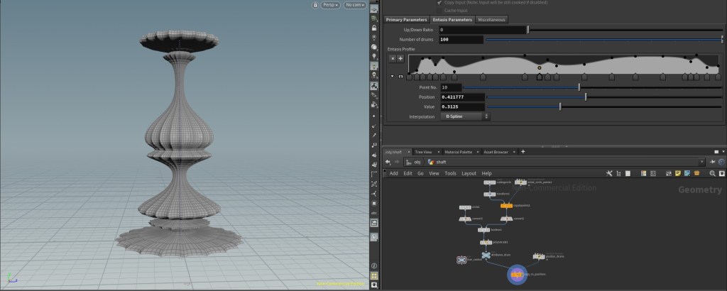
At first, in order to calculate the values of $radius_{current drum}$ and $radius_{next drum}$ , I directly implemented the rules described in the previous paragraph in the code. However, retrospectively, it was not a really good idea: changing the rules meant changing the code; you cannot expect artists to code and even for coders, it is nor fast, nor visual. Indeed, those architecture rules are made to achieve visual results (i.e make the column looks concave or convex or etc.) In that regard, finding a visual tool for defining the entasis would be better on both a design and scalability point of view.

I found out that Houdini proposes a nice tool for doing so: a ramp parameter (‘chramp’ if you want to search it in the documentation). Rather than giving the rule in terms of an algorithm, I used the ramp to directly draw the profile of the column, then the algorithm can find the values and create the corresponding column.

For example here is the Greek Doric profile: the slope is almost linear except in the first drums where it is more domed

The Roman Doric column is supposed to be straight at the first third of the column then has a linear shrink for the rest of the column: here is the corresponding ramp

Basically, you can read what the column would look like on the profile: your column is just the dark part (the bottom is on the left, you need to rotate it by 90 degrees). Here is the code if it interests you:

Here is a video showing how it works!

The ramp parameter controlling the entasis can be used to create more interesting shapes! Of course that’s quite a far-fetched way of getting those shapes I guess but that’s still visually interesting. At least I had fun playing with it 😀

I’m starting to realize the power of going procedural: by building tools ‘modular enough’, they can be used to create things useful in broader scopes than their original purpose. The ramp thingy is a pretty powerful tool when I think about it, you can directly ask the artist to draw a function and pass it as an argument which can have plenty of nice way to be used!

Now, we’re done with the entasis. In the next post, I will probably talk about subtilities about the curvature of Greek temple. Or trying to build an Ionic column.

PS: Here I propose a much simpler set-up for doing something similar. It is less detailed but much faster to implement and to run. For working in previsualisation and fast visual tests it might be useful!

Naive Doric Shaft

Let’s start simple and do ‘naively’ the modeling of the base column! We will improve it later in the next post! Let’s first review what we need to model before diving into Houdini.

The doric order is the one on the left (credits: Khan Academy)

As you can see the doric one is the most simple one and managing to do the shaft seems to be the easiest task so let’s start with that! Let’s first note that for the Greek Doric columns (which is not the case for the Roman Doric order!!), the column does not have a base, which means the shaft touches the stylobate (approximately the floor of the temple) directly.

The Parthenon in Athens with typical Doric columns (credits: Steve Swayne flickr)

The Doric column has merely the shape of a cylinder but as you can notice on the pictures, it is not smooth: the column is carved in what is called flutes. The reason of the fluting is not clear: from what I read, the main hypothesis are that it brings dynamic since it contrasts with the roundess of the column, or simply that it comes from the fact that previous columns were carved in the wood and then presenting this kind of ornaments.

The particularity of the Doric fluting is that it is sharp: there’s only one edge between each flute in contrast with Ionic flutes which present planes. Plus, Doric classicaly presents 20 flutes, when the other orders present 24. Strangely, it was extremely hard to find documentation on how the flutes were carved but I showed some obstinacy and found this picture:

Top cut of a doric column (Credits: *De re ædificatoria* (On the art of building, book III), Alberti, Leon Battista, 1485)

That’s small but that was enough for me to understand how I could do:

Create a circle of the desired radius (a)
Found the centers of the squares (as shown in the pic ^) (b)
Substract the circles with these centers as origin from the original circle (c)
Extrude (d)

So let’s do it now 😀 First let’s create an empty geometry and let’s dive into it.

(a) Create a circle of the desired radius

Obviously the easiest step. Just create a circle and create a Null node where we will stock our variables for user control:

(b) Found the centers of the squares

For this task I will use an Attribute Wrangle. An Attribute Wrangle is a node in which you can write some VEX code to do whatever you want. To understand how I could use the Attribute Wrangle I mainly used this blog page. If you’re not already familiar with coding, maybe Rohan Dalvi’s videos on Youtube can be a better choice.

Ok, so we’re gonna code, but what? I don’t like coding so I spend as much time as possible preparing what I want to do before coding it (so that I spend as little time coding).

Our goal is to find the centers of the squares as shown in the picture from earlier.

First step will be to find the coordinates of the orange dots (see figure below)

The orange dots are uniformly sampled along the circle (which means the angle between two dots is always the same and equals to $\theta = 2\pi / N$ radians -or $360/N$ degrees – with $N$ the number of desired flutes). If you remember your trigonometry, the next step is fairly simple:

Then, finding the center of the square is straightforward (or if you forgot your math, just believe me):

In the end, here is the VEX code that does the trick (feel free to copy it):

The result: the points seem to be at the right place

In order to do that, we will use a Houdini node called ‘Copy to Points’. Basically we will give him a Circle and our Points from the Wrangle and he will create a circle on each of those points:

Of course, that’s not what we want, we want to substract those circles from the original circle. In order to do so, we will: convert those circles into meshes then use a boolean operator to perform a substraction:

(d) Extrude

As the title says, we just extrude by adding a PolyExtrude node and TADAM we have what we wanted:

Houdini’s PolyExtrude node comes with interesting possibilities: we can create some Twist and Shrink (and creating global variables in our Null item to control it). Twist is more fun than useful but Shrink will be really helpful in next steps.

In the end we managed to create a column with the flutes that we wanted. In your Null object, we also have some nice variables to easily adapt our shaft:

So we’re done with our basic Naive Doric Column. In the next post, I will speak about entasis or why this is not satisfying yet! Follow the link 😀

About Salient Poses

When conducting my research on Keyframe reduction, my main starting point was the algorithm Salient Poses from a SIGGRAPH Asia Technical Brief (Optimal and Interactive Keyframe Selection for Motion Capture, Richard Roberts, J.P. Lewis, Ken Anjyo, Jaewoo Seo, and Yeongho Seol, SA 2018). In this article I will explain briefly what it is and how it works. For the point of view of the main author of the paper, please go check here

TL;DR

If you don’t have time, here is a quick summary of the algorithm:

Input: An animation (motion capture data -> curve in high dimension) plus an error function (takes a set of keyframes and computes how close the interpolation is from the real animation)

Output: the best set of exactly k frames for reconstructing the animation (for every possible k) aka the optimal set of k keyframes

How?: we use Dynamic Programming by iterating on the length of the animation! (First we make it stop at frame 2, then we push it further and further until we covered the whole animation) Complexity is polynomial.

Motivation: what do you mean by ‘Salient’?

Saliency is quite an important notion (and still so hard to describe properly) in data sciences and particularly in Computer Vision -I’ll try to write an in-depth article about that when I get some time.

Saliency is related to human cognition: the salient elements are the ones that attract the attention. For example, in an image, the salient element will be the closest object, in a video it will be the moving objects etc. such that it is easy to mistakingly think that Saliency boils down to object detection.

In animation, we see our animation as a curve -try to think of it as a motion trail- our goal is to find the Salient points of this curve which would be the most ‘notable’ points of the curve. The main goal of the paper is to perform keyframe reduction: from a motion capture input where there are keyframes everywhere, Salient Poses can reduce drastically the number of keys (keeping only 10%) without significant error in the animation such that the animation will be more convenient to edit.

The Salient Points of the curve would probably those points

An animation as a high-dimensional curve

First of all, the algorithm treats the animation as a ‘high-dimensional’ curve. Let’s start simple and imagine I am considering a simple ball moving. I can represent its movement by its motion trail (i.e the position of its center of gravity at any time) which describes exactly a curve -in dimension 3.

We track the 3 coordinates of our ball -> it is a curve in dimension 3!

Now, when considering a human moving it’s somehow more complicated. When you are looking at your motion capture data, you mainly have the translation of your root (or hips) which is like the ball from the previous example, but on top of that you need to add the rotation of all the joints.

In that regard, you can see your pose as a high dimensional point: you just need to concatenate the translate of your root and the rotations of all your joints.

However, one important thing to remember when working with high dimensional data is that the way you represent your data matters, even though different these representations might seem strictly equivalent to you.

When applying Salient Poses, rather than concatenating the rotations of the joints, we concatenate their position in space. The main reason we do that is that it helps getting our high dimensional points homogeneous: we only have position informations and not a mix of position, angles or quaternions. There are other pros and cons that I will try to cover here (the article is not ready yet, so no link for now :p).

The way we represent our pose when applying Salient Poses. Note that we use the transform informations (i.e the translate x,y,z) rather than the rotations of the joints

The error function

Another critical element of the algorithm is the error function. Basically the error function takes as argument a set of keyframes and will tell if reconstructing the animation using this set of keyframes will give a nice approximation of the original animation or not. If the value is low, it means that the set is good; if it is high, it means that the set is poorly chosen.

Left will have a high error value when right will have a low one as the keys are chosen more cleverly

To compute this error function, the original paper proposes to linearly interpolate between the chosen keyframes then compute the maximum distance between the linearly interpolated curve and the original one.

To compute the error, we construct the orange ‘linear interpolation’. Then we find the higher distance between the blue and the orange curve: it is our final error.

Please keep in mind that this is a design choice that was selected ‘experimentally’ but might (and need to) be discussed.

The algorithm

First of all, let me state what the algorithm solves. Given an animation and an error function, the algorithm will compute the sets of k keyframes that minimize the error function for every k possible.

How do we solve that? Of course, we can go brute force and test all possible sets but that will obviously be pretty inefficient. Good thing is we can use Dynamic Programming to solve this problem! (Brute force is exponential complexity, DP lets us get polynomial!)

As a reminder -or not- Dynamic Programming is a method for solving optimization problems and relies on dividing the problem in smaller subproblems.

In our case, the smaller subproblem is solving the problem for animations of smaller size: the idea is that, if I know how to solve the problem for the animation cropped at frame F, then solving the problem for the animation cropped at frame (F+1) is easy!

If I know how to find all the optimal sets of keyframes for left, then I can use those optimal sets to compute quickly the optimal sets of right!

For more details on how the algorithm performs at each iteration, please check the paper or this quick note I wrote for myself!

How do we use it?

The main use of Salient Poses is to implify Motion Capture datas. The main author implemented the algorithm into Maya: given an animation, it computes ‘quickly’ the optimal sets of keyframes. Then, the artist is free to check all those sets (there is some ghosting to display which poses would be chosen) then select the set that fits. The algorithm then performs simplification: it only keeps the keyframe of the chosen set and optimizes the tangents to keep an animation as close from the original as possible.

The orange dots represent a key: you can see that Salient Poses drastically reduces the number of keys but still manage an animation close to the original!

Discussion

There are really a lot of points that need to be discussed but I’ll give the most important ones here:

Evaluating: the main problem of this paper (and every single paper that covers keyframe animation to be honest) is the lack of metrics to evaluate properly the method. How can you say if a keyframe selection is good or not?

The error function: the paper proposes to compare the curve to the linear interpolation. It says that experimentally it gives better results than using spline interpolation or other interpolation method. However, once again, how can you evaluate properly the quality of these results?

The philosophy of the paper itself: so basically, the paper makes the initial assumption that the Salient Poses are the poses that would give a good interpolation. However this idea can be challenged as those two notions are from different scopes: Saliency relates to cognition when interpolation is more about computation. When you play a little bit with Salient Poses (I spent quite a few hours since I believe it is extremely interesting) you will notice that the algorithm will not necesarily pick the extremes, which is an heresy somehow. The reconstruction is still OK though, as it can use the tangents to optimize properly. So, we chose good poses for reconstruction but probably not Salient Poses in the end!

The good thing is, by playing on the error function, we can modify the criteria to have something more ‘topological’. The algorithm presented in the Salient Poses paper is powerful in the sense that it computes the optimal keyframe selection for the criteria that we proposed. However, it is up to us to provide a meaningful criteria.

There is still a lot of things to explore concerning this idea and, in my own opinion, I think there are extremely exciting ideas to develop. My first short paper (article incoming) proposes to use Salient Poses to solve some of its original flaws and my current work is still improving those results and giving them more interpretability!

Interpolating: Choosing the interpolation?

In this article, I’m gonna speak a little about interpolation. And why we mostly choose an interpolation scheme rather than another. So, as you would have guessed, the topic will be about mathematics in the first part and animation on second one (jump straight to animation if you do not care, but I promise, even the first part is easy to understand and really valuable!)

About Interpolation

A link between continuous and discrete representation

Let’s say I have a curve. A curve is continuous: you can draw it without lifting your hand. However, when we are doing animation, we do not consider the time as continuous anymore, we represent it as ‘keyframes’. If we want to represent how we moved on the curve, we would just put points at some places: a point means ‘I was here at that frame’. Representing something continuous as a countable number of points is called a ‘discrete’ representation

Going from Continuous Too Discrete. The curve is the continuous representation while the blue stars is a discrete representation

So, as we can see, it is pretty easy to go from continous to discrete, we just have to put points at the exat moment. In animation, even though the motion is supposed to be contiuous, we can represent it by still frames and the illusion of movement works if the framerate is high enough. So, in a way, animation is just a discretization of the movement

However, what if I give you points and ask you to draw the original curve? The question is way more complicated and sometimes impossible to do if there is not enough points, or if they are not distributed well enough.

Of course, it is impossible to find exactly the initial curve, we can always lose some level of details. But we can still hope to find something that is really similar to our initial curve. This process of approximating a continuous curve using a discrete representation of it (i.e points from the curve) is called INTERPOLATION.

OK, but how do we do that?

Note: for hands-on examples, go check the notebook I made especially for this topic: here

The first idea to solve this problem is fairly simple: let’s say I have points that are supposed to make a curve, how can I recreate that curve? Basic answer is: I just need to draw a line between each consecutive points. And that’s exactly what linear interpolation is!

Linear interpolation: we just draw a line between our points (it is a constant speed line!) The dotted line represents the initial curve that we want to approximate

As you may notice, given that we have enough points, the result is pretty good as it approximates well the initial curve. The more point we have, the closer we will be. But there is a huge problem. The curve that we constructed (the consecutive lines) is not smooth! It looks somehow geometric and not fairly natural. For multiple reasons (that I will cover in next section) we do not like that at all and want to avoid this non-smoothness! To do so we use ‘spline’ type interpolations (there are multiple sorts of splines) that allows us to recreate a smooth approximation of the curve!

The spline interpolation might not represent perfectly our curve, but it gives a fairly good representation which is SMOOTH!

About why spline is better than linear (in most cases)

Let’s talk physics

To understand what’s the point, we need some really basic notions of physics. Animation is all about physics after all!

In physics, when considering the movement of a point, we introduce two values that we find pretty valuable: speed and acceleration. Speed is how fast our point moves and the acceleration is ‘the speed of the speed’ i.e a positive acceleration means that the speed goes up so our point moves faster and faster, negative acceleration means the speed goes down so our points moves slower and slower.

On a graph representing, for example, the value of Translate Y of our point, we can read the speed quite easily. The speed is just the slope of our curve!

Imagine a ball falling, that’s what the plot of their Translate Y attribute would look like

Here is the graph representing its speed (the absolute value). When the ball falls, it goes faster and faster

The acceleration is just the ‘speed of the speed’. The ball accelerates but constantly (the value of the acceleration is 2 here, but it should be around 9.8 which is the value of standard gravity!)

Let’s analyze a linearly interpolated curve with that perspective

So let’s just draw a linear interpolation and check what is the speed of our point!

Here is the linear interpolation (in orange) between our points (in blue). The speed is just the value of the slope

The speed is constant on each segment so it basically looks like that!

You may notice something unusual: the speed is not continuous!!! Indeed, the slope brutally changes on each point we interpolated!

What is a discontinuity in the speed? It means that there is an infinite acceleration at that moment! And guess what? Infinite acceleration almost never occur in real life. In certain situations it can be acceptable (e.g robotic motion or bounces of a rigid body) as it is close to the phenomena, but most of the time it will not work and will result in an awkward feeling of the motion!

However, when using spline type interpolation, the result is smooth, and it is much better: we don’t have those discontinuities anymore!

Interpolating using a spline type interpolation

The speed of our point with this kind of interpolation. The result is not perfect, but still much better than earlier as there are no discontinuities!

In summary

Linear interpolation: it means constant speed! So if you need something that goes at a constant speed (robotic arm or elevator or such, why not!). But take care of tangent breaks!
Spline interpolation: smooth way to interpolate! It will make the transition smoother so that you will start to have an ‘ease-out’ and an ‘ease-in’! BUT rework your dynamics by yourself as the interpolation will not make it perfect!

Managing the camera when animating on two’s

With the success of the recent Spiderman Into the Spiderverse, animating on 2’s is becoming quite trendy. While it is quite an easy technique to do when the camera is not moving, it can become an horrible mess when the camera is moving and you do not know how to deal with it. There is a nice tuto on Youtube on how to perform this kind of things but it relies on a plug-in (which is not free). On multiple occasions, Sony Pictures’ animators talked about what they did (during a Production Sessions at SIGGRAPH LA 2019 or in an article from SideFX for example) and it’s not a super hard trick, but it’s pretty convenient to know. My goal here is to give a few details so that we understand exactly what happens.

Note: this article involves some extremely basic Python scripting. I will explain really in details so even if you are an absolute beginner in scripting it might be understandable! Oh, and it is done in Maya also. But that should not really be that different from one 3D software to another 😉

First, what is animating on two’s?

Animating on 2’s is a technique used in Spiderverse as I said earlier, but you can find it a lot in traditional and Japanese animation. It consists on drawing only one frame every 2 frame. When the framerate is usually 24 fps, it means that we will have only 12 frame every second. However, it is not just a downgrade in the framerate. Most of the time, the camera still continue to move in 1’s (so keep the 24 fps rate), but the character move on 2’s.

Let’s go hands-on

For the sake of this explanation I will use an old walk cycle that I did a few months ago. I animated in 1’s so we will first need to put it in 2’s (*)! We will see what is the problem with the camera work and how to fix it.

So, according to what I said before (and the figure explains it well), you just need to remove one frame every 2 frames. However, most of the time, we don’t put keyframes on EVERY frame and on every controller, we often rely on interpolation. An easy way to deal with that problem is to use the ‘bake keys’ function (**).

Select ALL the controllers of your character
Go in Key/Bake Simulation (if you do not have the tab Key, change your mode to “Animation”)

Ok, so what did it do? Basically, it just went through all your animation and put keys everywhere. So your animation is in 1’s exactly like in the picture from last paragraph. Ok, so now, we need to put it in 2’s. You could just manually remove delete a keyframe every 2 frames (***); it works but that’s really boring and somehow long. We can use a basic Python script for that. The role of a script is to give instructions to the software so that it can perform repetitive tasks at your place (and then, really fast).

First, select all your controllers (you need to make sure all your controllers will still be selected when running the script), then, open your Script Editor. Start coding:

import maya.cmds as cmds
import maya.mel

selection = cmds.ls(sl=1) #selection is exactly supposed to store what you have selected
frameStart=0 #the first frame of your animation, in my case it is 0
frameEnd=130 #the last frame of your animation, in my case it is 130
for t in range(frameStart,(frameEnd-frameStart)//2): #for every frame in the animation
    cmds.currentTime(2*t+1) #I go to every odd frame 
    maya.mel.eval('timeSliderClearKey') #and suppress the keys

Ok, everything is written in the comments but let me just explain real quick. The first two lines is just for preparing your software (your Python interpreter to be more precise) that you will use some of Maya functions. In the next block, the first line is for saying that the variable ‘selection’ contains what you have selected (i.e all your controllers if you did what I told). Then, you go through every frame of your animation (2*t are the even frames, and 2*t+1 are the odd ones) and deleteKeys of the odd frames. And that’s all!

Let’s take a look! I first show the animation on 1’s, without camera motion, then with camera motion. Then I show the same animations on 2’s.

(*) Animating in 2’s by taking an animation in 1’s and ‘downgrading it’ is pretty much a bad idea. If you want to animate in 2’s, you need to think in 2’s. The thinking process about the overall dynamics might be the same but you also might have considerations like finding stronger poses, techniques you would use-smears if one to mention- and when to put them, even before animating. But I still do that for educative purpose-and because I do not have enough time and enough skills to do a full animation in 2’s quickly.

(**) If you know a little bit what’s happening in Maya, you don’t want to use that, since it will be very slow. Better work directly with the animation curves so that you don’t have to use anything that update the time and evaluate all the nodes all the time. But the code is way more basic and clear written that way 😉

(***) Removing the odd frames is probably not optimal and somehow arbitrary. What if my keypose is on the odd frame and the frame just before (and after) are just inbetweens? My animation will definitely lose some impact. Part of my research is dedicated to give a relative importance to frames so that might give better practices for that point.

IT’S HORRIBLE, WHAT HAPPENED??

The animation, without the camera movement seems OK though, there is that choppy style which is characteristic of animations on 2’s. But when there is the camera movement it is really really bad. The character is giggling and it’s annoying to watch. So what’s happening exactly?

The eye represents the camera, the duck represents our character. On 1’s the duck and the camera moves at the same speed so the duck stays at the center. But on 2’s, since the camera moves on 1’s but not the duck, the duck is stuck where it was before!
It creates a back and forth movement since the duck is late/right timing/late/right timing/late… again and again and again, and that’s really uncomfortable to watch.

Since our camera is moving the correct way, but not our duck (or our Spinosaurus), no wonder why our movement looks strange, especially with that back and forth. But why does it work in Japanese animation for example?

Check this example. The movement of the camera is crazy, too crazy, the character is obviously not on 1’s but that’s still working and not only that, but the result is extremely fluid and really cool. If you go frame by frame or just scroll slowly the time bar, you will notice that the character is locked on screen. During their presentation at SIGGRAPH, Sony’s animators were using a formulation like ‘pixel locked’: on the frame that our character does not move, it still needs to remain at exactly the same pixels on camera, even though the camera changes! In 2D it’s a natural thing to do but not in 3D!

Let’s pixel lock our character: First Attempt

So, how can we do that? First answer would be, ‘you want to lock my camera on screen? Then, just constrain the character to the camera!’ That’s a fair and simple answer, let’s try!

That looks good! But is it what we want? Definitely no!

We lost the movement of our camera!! If you watch the initial animation, the camera gets further and further away from our character! Here, the animation is locked, but in the initial position of the animation!

Constraining is not dumb, but what we should do is to apply multiple constraints! One every two frames to be precise. Here is how we should do it:

The red line is the original animation. Every odd frame should stay on that animation, but we should just follow the movement of the camera for the frame the pose is not changing!

Second (and last) Attempt

Now, we somehow understand what we have to do. We should just move our character ONLY on the frames they’re not changing (every odd ones for examples), and by the right amount so that they’re locked on screen.

Setting tons of constraints is a boring idea, so we will do a quick and efficient script instead.. But first let’s just check how we need to move our character to lock them.

It’s pretty simple. If we make a pure translation (left) for our camera, we just need to translate our character by the same amount. If we make a pure rotation, we somehow have to make the same rotation for our character (plus a rotation taking the camera as the pivot)

Here is the Python code (don’t worry too much about the add function, I’m using numpy for computations but you probably won’t have that installed in your Maya so I needed to get a quick solution)

import maya.cmds as cmds #import the maya functions

#we create a function add to add/substract lists such that: (a,b,c)+(1,2,3)=(a+1,b+2,c+3)
def add(list1,list2,substraction=False):
    if(len(list1)!=len(list2)):
        print('Not same length!')    
    coeff=1.
    if substraction:
        coeff=-1.        
    for i in range(len(list1)):
        list1[i]+=coeff*list2[i]
    return list1

cameraName='camera2' #we get the name of our camera
selected = cmds.ls(sl=1) #select the MAIN or root of your character

for t in range(65): #it was 65 in my case, (frameEnd-frameStart)//2 for you
    cmds.currentTime(2*t) #we go to the even frame
    original_cam_transform=cmds.xform(cameraName,q=True,ws=True,t=True) #to check the position of the camera
    
    cmds.currentTime(2*t+1) #we go to the odd frame
    new_cam_transform=cmds.xform(cameraName,q=True,ws=True,t=True) #we get the new position
    translation = add(new_cam_transform,original_cam_transform,True) #we calculate the difference ie the amount the camera moved
    
    selected_transform=cmds.xform(selected,q=True,ws=True,t=True) #we get the current value of our selection
    new_selected_transform=add(selected_transform,translation) #we move it by the amount the camera moved
    cmds.xform(selected,ws=True,t=new_selected_transform) #we give this value to our selection

Note: If you look at the code closely, you will notice that I only work the translations! In my scene I only have translations so I did not need to care about if the camera rotates or not. But it is not way more complicated, you would just need to work with Transformation Matrices rather than just adding stuff, it is way more clear written only with translations. Reach out to me if you need to do some rotatoes 😉

So, here is the final result:

Of course there are tons of other things to do to improve the results (selecting the keyframes more cleverly or PLANNING to animate in 2’s from the start) But I hope you got the idea! Just lock your character in screen on the freezed frames!

This is not the only way of achieving that! You can for example try, during the rendering, to get separate AOVs for the objects and the background and keep only 1/2 frame for the objects that will be in 2’s.

The advantage of the technique I described is that it is more flexible: by tweeking the code you can choose on which frame you want to apply the pixel lock (so that you can easily choose where you want to animate on 2’s or on 1’s if you want to mix the styles!)

Let’s overlap!

Overlap is quite a common principle that brings a nice organic feeling to the movement! It is particularly efficient when dealing with extremal limbs such as arms, tails or animals’ ears… With no more talking, let’s get started!

A first basic example!

As I said earlier, overlaps is especially efficient when working with tails, so imagine I have a dino and I want to move his tail up and down (cf. images below). In order to do so, I will create 4 keyframes, one for the initial pose, one for the pose where the tail is down, one for when it is up and finally one for going back to the initial pose.

We put exactly the same pose on the beginning and the end of the animation so that it can loop! We use directly spline interpolation between the poses! (Credits: Spinosaurus rig by TRUONG)

The result is OK but not really convincing, the tail of our dino seems a little bit stiff and the movement is somehow robotic. Let’s take a look at the graph editor to see what’s happening.

If you watch the curves representing the rotation of the joints of the tail, you see that all the rotations are synched!

That synchronization may be a problem (I will give an intuition of why is that in the last paragraph!). Let’s just desynchronize by offsetting all the rotations by 2 frames from each other: we obtain the graph below as result

We can even push by taking an offset bigger, like 4 frames! Let’s take a look at the result:

Without effort we have a result that is already way less robotic and seems more flexible! Of course, there are other things to improve that movement (working on the amplitude and the timing to lose that “too symmetric” feeling that we have for example) but that’s not the point of this talk 😉

Just playing with the moment the rotations (or the movements of the joints) are engaged can remove the feeling of stiffness that we have if everything move at the same time.

Let’s have another example

Though the trick worked here, I don’t want you to think that the only way of doing overlap is by creating your poses then offsetting everything afterwards. To be honest, it’s not really a good practice (but it works so use it when you can!) as it creates a lot of keyframes everywhere -and not the same for every controller- so that can create quite a mess.

In animation, it is always better to ‘know what you’re doing’. Rather than recklessly moving our frames afterwards, it is way better to use the breakdowns to prepare our movement so that the overlaps are controlled! Let’s take the punch animation from this video.

Only look at the final result 😉

So what we have to do is just putting a breakdown on Frame 8 to notify that we don’t want to move the second rotation until 8! And miraculously, the interpolation gives a nice result 😀

Idem for when the arm will punch the table! The arm extends only at the frame before the punch (it’s a way of giving more impact also). Just put a breakdown on 34 to say that we do not want the rotation to start yet and you are good to go.

In the end, it is somehow the same process than in the previous section, except that in this case, we used our brain and had more control over what we were doing!

Why is it so important to engage the joints at different timing??

My explanation is not totally accurate as there are multiple categories, but gives a nice intuition about what is happening. As we saw earlier, giving engaging all joints at the same time results in a robotic/stiff/rigid motion.

In physics, we call ‘rigid bodies’ solids that cannot be deformed. What does it mean for these rigid bodies? A particularity they have is that every particles they contain somehow move all the same way (to be precise they keep the same relative distance with regards to each other). If it only translates, all the particles will have the same speed; if it only rotates, they will all have the same angular velocity.

But most of the things we are considering in the real world are not rigid bodies. For example, that’s why, when you animate the flesh (during polishing step), you will probably make it wiggle with a short delay compared to the primary animation.

Furthermore, when you lift naturally your arm, you will mostly put your energy for lifting your upper arm, then, the speed your forearm will get from the beginning of the movement will make it easier to lift it afterwards! Engaging everything at the same time (except in some cases of course) is not natural because it’s not efficient at all!

If there is something to remember from this post, it is to deeply think about your movement before animating it! If you understand how your character handles its energy and how they uses their limbs, you will engage the movements of the different joints at the right timing and get natural overlaps!

Cheers,

Nico

A few precisions about Computer animation

In this article, I will briefly talk about the basics of Character Animation in Computer animation so that we can quickly get an idea of how animators work inside their animation software! This talk is slightly more technical than the one about animation but nothing really crazy. It’s not totally exact either, but it is simplified so that it is easy to understand.

What is the equivalent of drawing in 3D?

If you already read the article about the basics of animation, you would know that we need to first craft ‘keyframes’ and ‘breakdowns’. In 2D that’s pretty obvious, we need to draw, or on a piece of paper that we will scan, or directly on softwares like Photoshop. In CG (Computer Graphics), it’s a little bit more complicated.

First, we need to create a 3D Model of our character (that’s a step called ‘Modeling‘). In CG, 3D models are just a huge piece of geometry composed of ‘meshes’, indeed, if you look very closely your 3D models, it’s not totally smooth but rather a concatenation of small polygons*.

(*) There is a ‘smooth’ way to represent 3D shapes called ‘implicit surfaces’ but that’s somehow complicated -basically, we represent the shape as the solution of a given equation- and a whole topic of research so let’s not talk about that here 😉

A 3D model is nothing but tons of polygons put together (credits: Mixamo model courtesy of Adobe)

So how do we make it move?

Do we need to move all the vertices one by one to shape our poses then? That would be really really painful and not such a good idea. Instead, we create a skeleton that we link to our 3D model. Moving the skeleton will move the geometry accordingly so we do not have to care about the mesh anymore and can rather focus on the bones.

We can manipulate the skeleton (in purple) rather than working directly on the geometry

In practice, most of the time, we do not even touch the bones directly, we prefer creating manipulators that will control the bones: we obtain some sort of puppet that we can manipulate easily and then shape our pose comfortably.

Each curve around the character are controllers that ‘control’ a different part of the body, they do not have the same effect. When clicking on a controller, the arrows (on the right pic) will appear and will let manipulate the character interactively. (Credits: Cyborg Rig by TRUONG)

We can also apply rotations. In this case, we click on the shoulder controller, go in rotation mode then rotate using the rotation manipulator

By manipulating our puppet, controller by controller, we can finally make our pose quite instinctively. Easy right?

We call this puppet a ‘rig’ and the process of creating such a rig from a 3D model is called ‘rigging’ (it involves an extra step called ‘skinning’: we need to make sure that the geometry of the 3D model deforms correctly when manipulating it)

A few (not so) technical details

Let me clarify what I said earlier. When we modify the controllers, to be more precise we modify its ‘attributes’. For example, the most common attributes are the values of the ‘Translation’ and the ‘Rotation’ which indicate how much the controller is tranlated/rotated from its initial position.

When we translate the Hips by 10 on the Z axis (i.e we move by a distance of 10 on the right)., the attribute ‘Translate Z’ increases by 10.

To summarize, when we manipulate the rig, we change the value of some of its attributes. From the values of the attributes, the rig can calculate how the geometry of the 3D model will be. (When you think about it, if the rig is really complicated, it will not be possible to calculate fast enough to achieve real time manipulation. That’s why some rigs have some latency when manipulating them)

And what about the interpolation?

When you think in terms of attributes, the interpolation is really straightforward, you just have to move slowly your attribute to its value from one pose to the values of the other poses.

To make it clearer, let me give you a concrete example. Let’s say I have a cube that moves only on the Z axis (from left to right or right to left only. It cannot up/down forward/backward). Consequently, it has just one attribute: its Translate Z. I want it to be at Z=0 on frame 1 and Z=10 at frame 50.

I represented the Graph showing the value of Translate Z in function of the time (i.e which frame we are). Since we are in ‘blocking’, it stays at 0 and brutally switch to 10 at frame 50

Now, you must see what I mean, rather than brutally switching the value, why don’t we make it change over time? In mathematics it is called ‘interpolation‘: we find a smooth transition to go from one value to the other. The value of Z over time is an object that we call ‘animation curve‘. To interpolate (create the inbetweens) the movement of our rig, we just have to interpolate the animation curves of each of its attributes!

After interpolation, we see that the value of Z changes over time. As a result, the cube moves also gradually!

Conclusion

I tried to cover the very basics in this article. To sum up:

We create a 3D model which is a chunk of polygons
We create a ‘RIG‘ which lets us manipulate the 3D Model as a puppet
When we manipulate the rig, in reality, we are updating the attributes of the rig. The rig uses these attributes to calculate the pose
To interpolate between the poses, we just interpolate the animation curves i.e the values of the attributes over time

I will tackle more notions about manipulation (IK/FK manipulation, blendshapes etc.) in further articles. If this one was not clear already, please contact me, I will do my best to improve this article!

Cheers,

Nico

Short brief about Character animation

The goal of this article is not to give a complete explanation about what is animation or how to animate, it is a way too broad topic and a lot of people already covered it way better than me (if you want, check Richard Williams’ book ‘The Animator’s Survival Kit’ which is a reference amongst animators)

My point is to explain quickly, basic notions of animation, so that it will be easier, for people with no animation background at all, to understand my upcoming articles. But since I come from a scientific background and have, in that regard, quite an analytic point of view, I hope I can still bring to the table things that can be interesting for artists.

Let’s start really basic

First of all, what is animation? It could be considered as the art of giving life (anima in Greek means ‘life’, ‘soul’) to static images. Indeed, most of the animation techniques consist of drawing/taking multiple pictures -that we call frames- that are slightly moving, then projecting them fast enough to give the impression of the movement. We call the frequency of this projection framerate: a framerate of 24 frame per second (fps) means that we show 24 frames in one second.

So, in a way, animating seems pretty simple, you just have to draw your character every 0.04s (24 fps) and that’s all. Except that if you try it, you will understand that it is not so easy. On a side note, it is not impossible, some animators work like that, it is called Straight Ahead animation but it is highly discouraged for beginners.

The usual ‘blocking’ workflow

If you still try to animate straight ahead like a maverick -I started like that actually- you will quickly notice a few things. There is a high chance you will not know what you are doing and where you are going. And even if you know where you want to go, you will probably not get to the pose you wanted initially, and at the right timing.

To solve this issue, animators work with something they call keyframes. The keyframes, as their names suggest, are frames that are key to describe the movement; with only these frames you should already be able to understand the motion. The animator craft or draw the keyposes and give them a timing (i.e choose the frames where they will be shown) to produce a ‘blocking‘.

(check the video far below to see the resulting animation) With these 3 frames we somehow understand what is happening: there’s someone hitting a table

Then, we create other poses that we call ‘breakdowns‘, their role is to precise the spacing i.e give information about the dynamics of the movement. For example, do I go to one pose to another at constant speed or by accelerating? by going straight or doing an arc? etc.

(check the video below to see the resulting animation) Top are the breakdowns (BD) that we added. BD1 & BD2 indicates that we slowly accelerate then decelerate to go from Pose1 to Pose2. BD3 & BD4 show that going from Pose2 to Pose3 is brutal and only take a few frames.

After we put enough breakdowns, we can focus on giving some smoothness to the motion. In 2D, it will consist of drawing the ‘inbetweens‘ i.e the frames between each breakdowns/keyframes. In 3D, we call it ‘spline‘, we let the computer calculate those frames -with a method called spline interpolation- between each of the poses we crafted. However, in both cases, it is not really straightforward and requires some work: we are not sure that the interpolation will behave how we expect it to do and some cleaning will probably be highly necessary. In his book, Richard Williams even states that (even though it is often done in practice), animators should do the inbetweens themselves and not let this task to the assistants as the assistants -somehow like the computer- would not do it properly.

Finally, there is an extra step of ‘polishing‘: it is time to correct some poses/timing/spacing, add extra details to make the result even more pleasant to watch. For example, in the video below, I increased the overlaps, added an anticipation and an overshoot/bounces to convey more strength in the impact. I will tackle all those subjects in upcoming articles 😉

https://vimeo.com/355817497 (if the embedding do not work)

Let’s summarize

To animate, we need to produce still images that we will read at a given framerate (generally 24fps)
First, I will work on my posing: WHAT are the actions that I want to describe
Then, I will give a TIMING to my poses: WHEN (at which frame) do these actions take place
It’s time to add breakdowns to set the SPACING: HOW I go to one pose to another, which trajectory/dynamics etc.

A few comments before ending this short introduction.

I did not mention the first and most important step which is the preparation of the shot. It is basically answering all those questions above (What/When/How) plus Why. Answering these questions is absolutely crucial as it is deeply linked to the storytelling role of the animators -and the reason why they cannot be easily replaced by a dynamics solver. Every pose/timing/spacing is an answer from the animator to one of those questions. When taking any decision, animators somehow need to always think about what they want to convey: when I’m making this pose, do I want to make my character seems reliable or suspicious? When crafting that timing, do I want them to look happy or gloomy? Setting that spacing, do they feel energetic or tired? etc. It’s the result of a thinking process on a micro scale (respect the physics/dynamics) and on a macro scale (respect the personality/mood/story). And that’s why it is so hard and complex I do believe.

Furthermore, remember that this is the usual workflow but not the only way of animating. There is the straight ahead approach, but you can also animate directly in spline: the purpose of this way of working is to shape as soon as possible the dynamics/timing (and then the rythm) of the shot and to work on the poses later on, it is particularly efficient on some action shots where the tempo is everything!

Hope you liked it! For any concern, question, correction, please tell me in the comments or by mail, I’d be happy to discuss anything regarding that topic!

Cheers,

Nico